Understanding the task
The goal of object detection is to recognize instances of a predefined set of object classes (e.g. {people, cars, bikes, animals}) and describe the locations of each detected object in the image using a bounding box. Two examples are shown below.
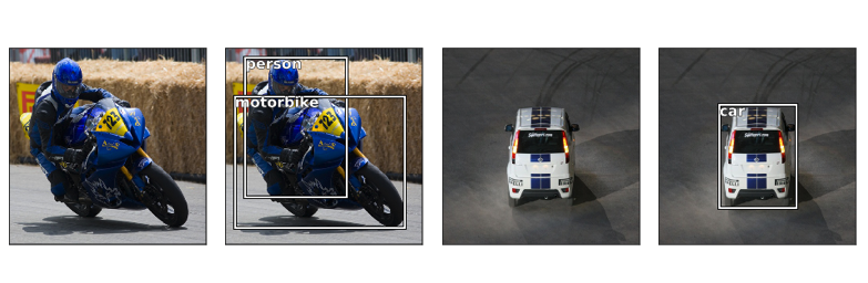
Example images are taken from the PASCAL VOC dataset.
We'll use rectangles to describe the locations of each object, which may lead to imperfect localizations due to the shapes of objects. An alternative approach would be image segmentation which provides localization at the pixel-level.
One-stage object prediction
Predictions on a grid
* backbone network: pre-train된 CNN(image classifier)에 이미지를 넣어 feature 추출
- image classification은 하나의 label만을 필요로 하므로 쉬움 (각 이미지에 bounding box annotation을 정의하는 것에 비해)

* backbone network에서 마지막 몇 layer만 삭제 -> 각각의 feature map들은 원본 image의 각기 다른 feature를 나타냄
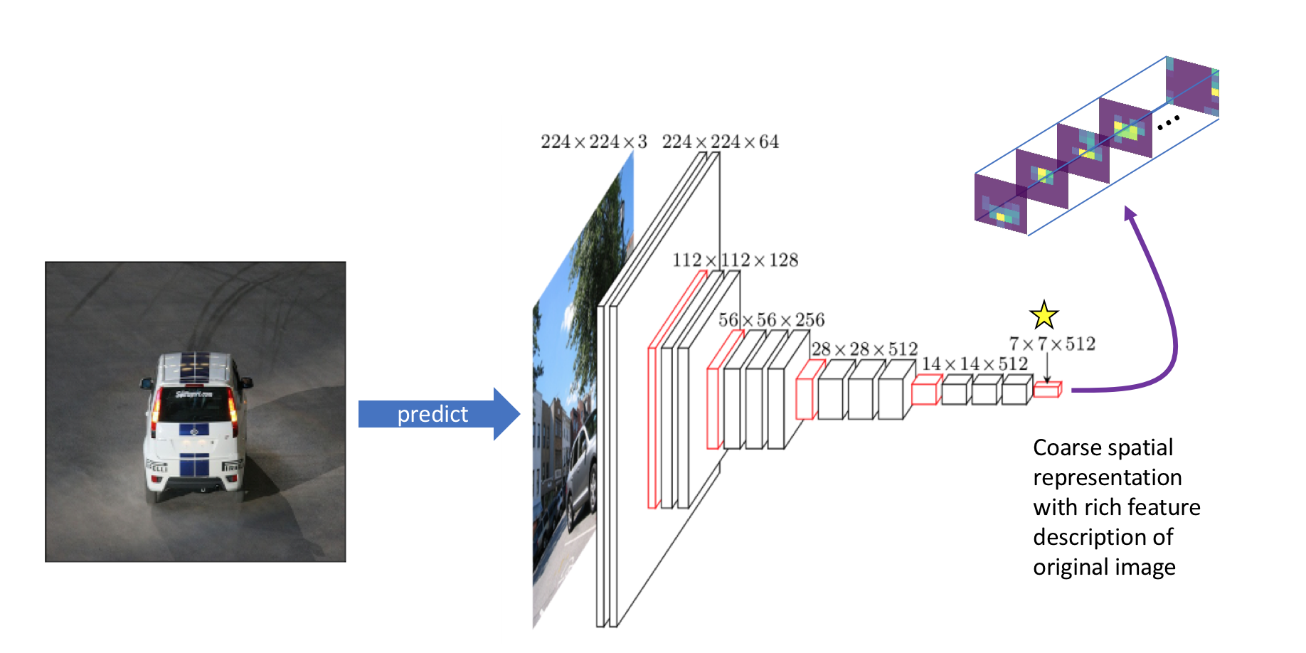

* 이 최종 feature maps는 grid들로 이루어짐 (여기서는 7x7) -> 원본 image 상의 어떤 feature를 나타냄
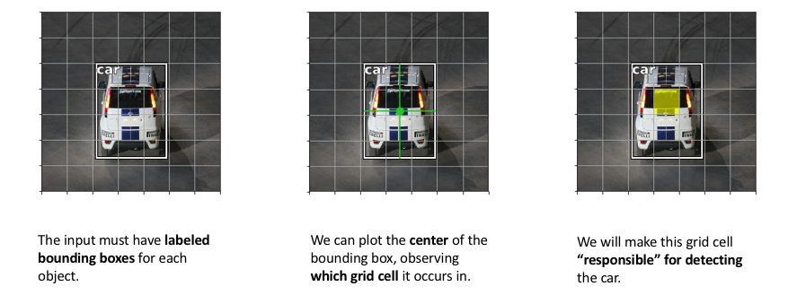
* "responsible" grid cell: 7x7 grid cells 중 bounding box의 center를 포함하는 것
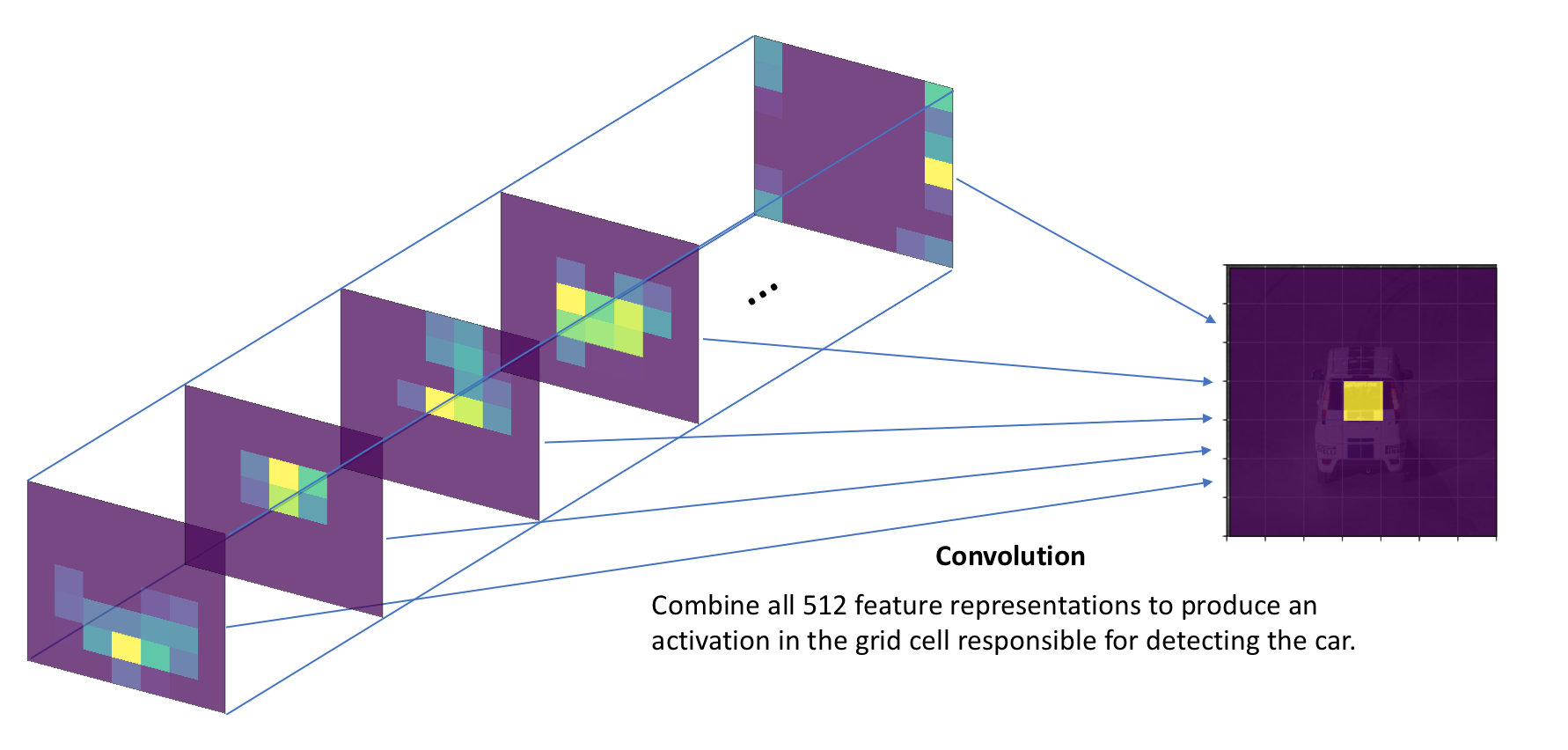
* 추가적인 CNN을 통해 모든 (여기서는 512개의) feature map들을 combine -> 찾고자 하는 object를 갖고 있는 grid cell의 activation 생성
- 찾으려는 object가 여러 개라면, activation도 여러 개여야 함

* 그런데, activation 하나만으로는 한 object를 충분히 설명할 수 없음
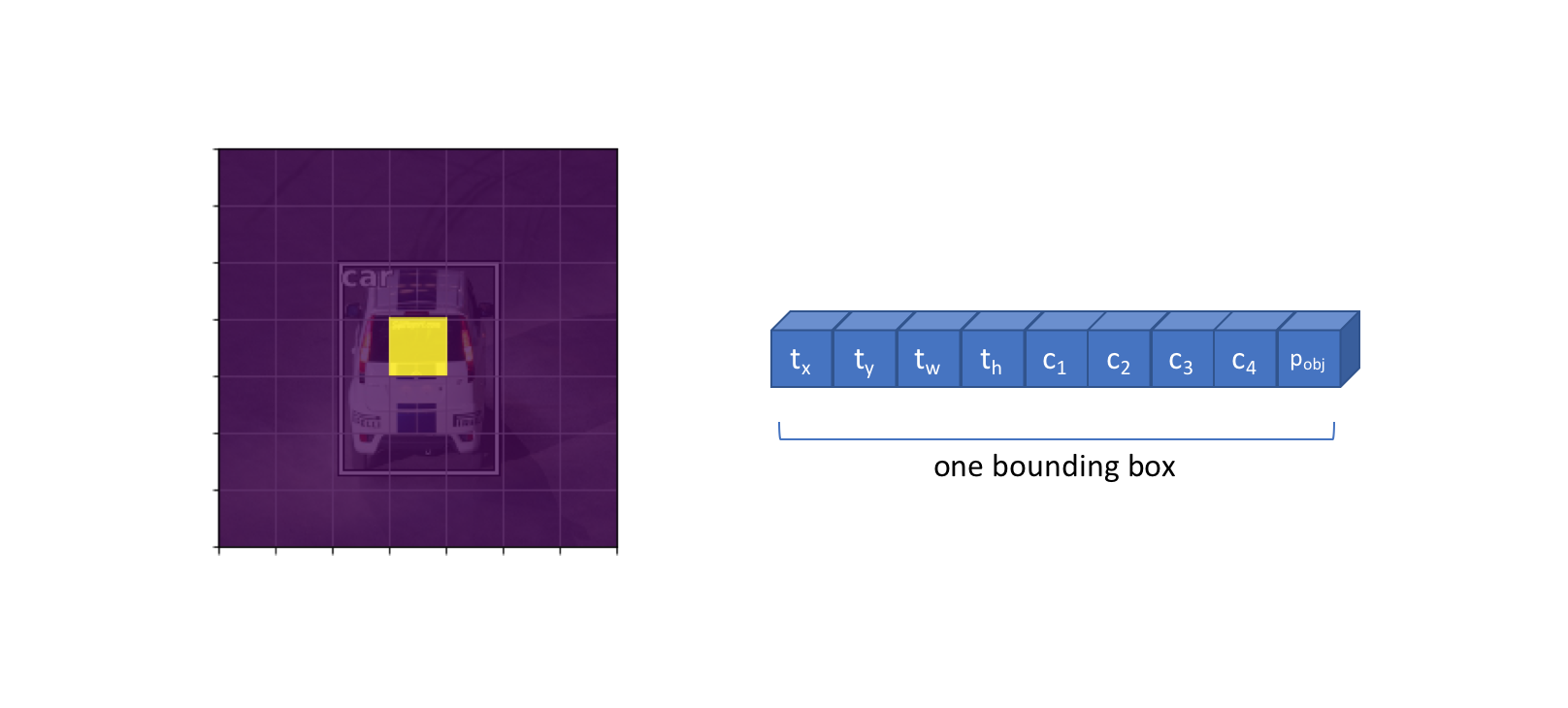
* 따라서, 총 (5+C)개의 출력 channel을 생성해야 함 -> 각 channel마다 하나의 convolution filter를 train시켜야 함
: 한 grid cell의 single bounding box를 설명할 수 있음
-> 어떤 grid cell이 특정 object를 포함할지, 각 grid cell에 어떤 class가 존재할지, 각 grid cell에 있을 수 있는 object를 결정할 수 있음
- p_obj: 이 grid cell이 어떤 object를 포함할 likelihood
- t_x, t_y, t_w, t_h: bounding box의 descriptors
- c_1, c_2, ..., c_C: 그 object가 어떤 class에 속하는지 (아마 one-hot encoding?)
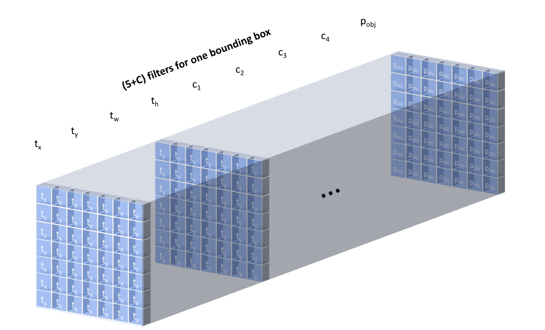
This means that we'll learn a set of weights to look across all 512 feature maps and determine which grid cells are likely to contain an object, what classes are likely to be present in each grid cell, and how to describe the bounding box for possible objects in each grid cell.
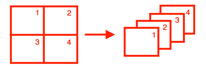
The full output of applying 5+C convolutional filters is shown below for clarity, producing one bounding box descriptor for each grid cell.
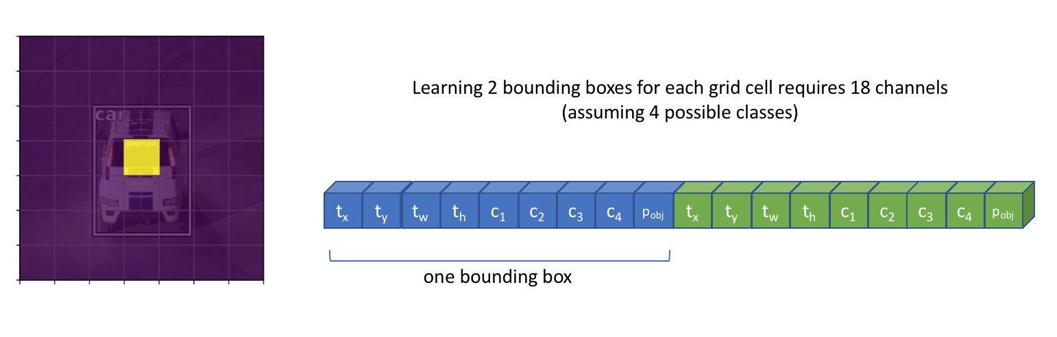
However, some images might have multiple objects which "belong" to the same grid cell. We can alter our layer to produce B(5+C) filters such that we can predict B bounding boxes for each grid cell location.
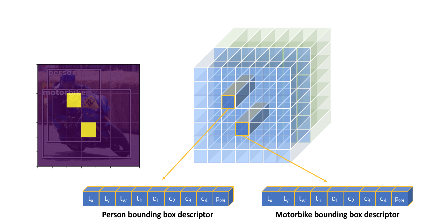
Visualizing the full convolutional output of our B(5+C) filters, we can see that our model will always produce a fixed number of N×N×B predictions for a given image. We can then filter our predictions to only consider bounding boxes which has a p_obj above some defined threshold.

Because of the convolutional nature of our detection process, multiple objects can be detected in parallel. However, we also end up predicting for a large number grid cells where no object is found. Although we can filter these bounding boxes out by their ���� score, this introduces quite a large imbalance between the predicted bounding boxes which contain an object and those which do not contain an object.
The two models I'll discuss below both use this concept of "predictions on a grid" to detect a fixed number of possible objects within an image. In the respective sections, I'll describe the nuances of each approach and fill in some of the details that I've glanced over in this section so that you can actually implement each model.
Non-maximum suppression
The "predictions on a grid" approach produces a fixed number of bounding box predictions for each image. However, we would like to filter these predictions in order to only output bounding boxes for objects that are actually likely to be in the image. Moreover, we want a single bounding box prediction for each object detected.
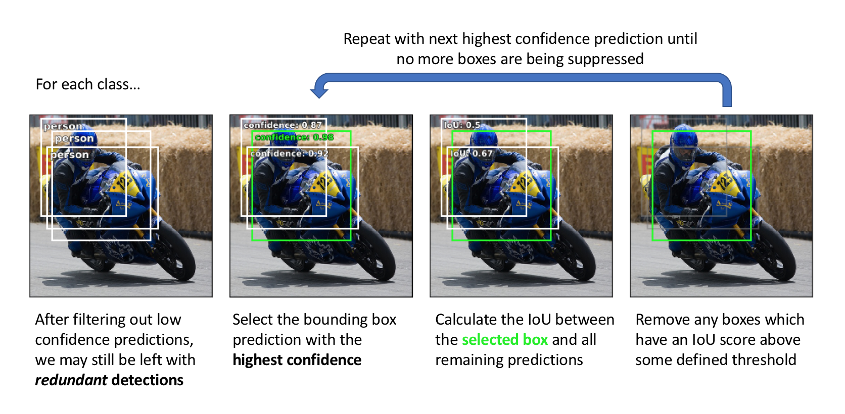
We can filter out most of the bounding box predictions by only considering predictions with a p_obj above some defined confidence threshold. However, we still may be left with multiple high-confidence predictions describing the same object. Thus, we need a method for removing redundant object predictions such that each object is described by a single bounding box.
To accomplish this, we'll use a technique known as non-max suppression. At a high level, this technique will look at highly overlapping bounding boxes and suppress (or discard) all of the predictions except the highest confidence prediction.
We'll perform non-max suppression on each class separately. Again, the goal here is to remove redundant predictions so we shouldn't be concerned if we have two predictions that overlap if one box is describing a person and the other box is describing a bicycle. However, if two bounding boxes with high overlap are both describing a person, it's likely that these predictions are describing the same person.
YOLO: You Only Look Once
Backbone network
The original YOLO network uses a modified GoogLeNet as the backbone network. Redmond later created a new model named DarkNet-19 which follows the general design of a 3×3 filters, doubling the number of channels at each pooling step; 1×1 filters are also used to periodically compress the feature representation throughout the network. His latest paper introduces a new, larger model named DarkNet-53 which offers improved performance over its predecessor.
All of these models were first pre-trained as image classifiers before being adapted for the detection task. In the second iteration of the YOLO model, Redmond discovered that using higher resolution images at the end of classification pre-training improved the detection performance and thus adopted this practice.
Adapting the classification network for detection simply consists of removing the last few layers of the network and adding a convolutional layer with �(5+�) filters to produce the ��� bounding box predictions.
Bounding boxes (and concept of anchor boxes)
The first iteration of the YOLO model directly predicts all four values which describe a bounding box.
The � and � coordinates of each bounding box are defined relative to the top left corner of each grid cell and normalized by the cell dimensions such that the coordinate values are bounded between 0 and 1. We define the boxes width and height such that our model predicts the square-root width and height; by defining the width and height of the boxes as a square-root value, differences between large numbers are less significant than differences between small numbers (confirm this visually by looking at a plot of �=�). Redmond chose this formulation because “small deviations in large boxes matter less than in small boxes" and thus when calculating our loss function we would like the emphasis to be placed on getting small boxes more exact. The bounding box width and height are normalized by the image width and height and thus are also bounded between 0 and 1. An L2 loss is applied during training.
This formulation was later revised to introduce the concept of a bounding box prior.
Rather than expecting the model to directly produce unique bounding box descriptors for each new image, we will define a collection of bounding boxes with varying aspect ratios which embed some prior information about the shape of objects we're expecting to detect. Redmond offers an approach towards discovering the best aspect ratios by doing k-means clustering (with a custom distance metric) on all of the bounding boxes in your training dataset.
In the image below, you can see a collection of 5 bounding box priors (= anchor boxes) for the grid cell highlighted in yellow. With this formulation, each of the � bounding boxes explicitly specialize in detecting objects of a specific size and aspect ratio.
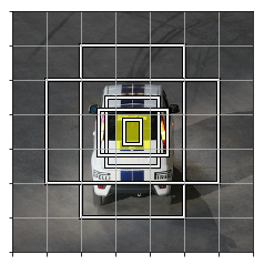
Note: Although it is not visualized, these anchor boxes are present for each cell in our prediction grid.
Rather than directly predicting the bounding box dimensions, we'll reformulate our task in order to simply predict the offset from our bounding box prior dimensions such that we can fine-tune our predicted bounding box dimensions. This reformulation makes the prediction task easier to learn.
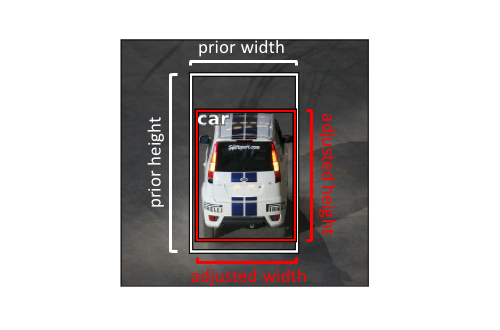
For similar reasons as originally predicting the square-root width and height, we'll define our task to predict the log offsets from our bounding box prior.
Objectness (and assigning labeled objects to a bounding box)
In the first version of the model, the "objectness" score ���� was trained to approximate the Intersection over Union (IoU) between the predicted box and the ground truth label. When we calculate our loss during training, we'll match objects to whichever bounding box prediction (on the same grid cell) has the highest IoU score. For unmatched boxes, the only descriptor which we'll include in our loss function is ����.
After the addition bounding box priors in YOLOv2, we can simply assign labeled objects to whichever anchor box (on the same grid cell) has the highest IoU score with the labeled object.
In the third version, Redmond redefined the "objectness" target score ���� to be 1 for the bounding boxes with highest IoU score for each given target, and 0 for all remaining boxes. However, we will not include bounding boxes which have a high IoU score (above some threshold) but not the highest score when calculating the loss. In simple terms, it doesn't make sense to punish a good prediction just because it isn't the best prediction.
Class labels
Originally, class prediction was performed at the grid cell level. This means that a single grid cell could not predict multiple bounding boxes of different classes. This was later revised to predict class for each bounding box using a softmax activation across classes and a cross entropy loss.
Redmond later changed the class prediction to use sigmoid activations for multi-label classification as he found a softmax is not necessary for good performance. This choice will depend on your dataset and whether or not your labels overlap (eg. "golden retriever" and "dog").
Output layer
The first YOLO model simply predicts the ��� bounding boxes using the output of our backbone network.
In YOLOv2, Redmond adds a weird skip connection splitting a higher resolution feature map across multiple channels as visualized below.
The weird "skip connection from higher resolution feature maps" idea that I don't like.
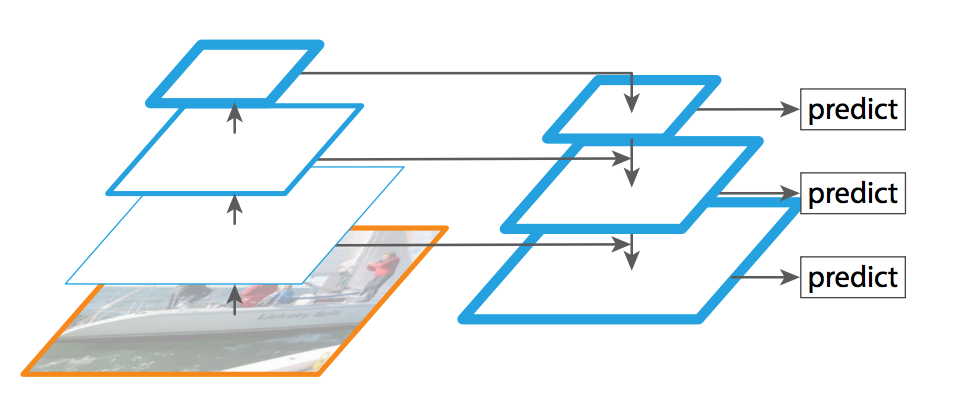
Fortunately, this was changed in the third iteration for a more standard feature pyramid network output structure. With this method, we'll alternate between outputting a prediction and upsampling the feature maps (with skip connections). This allows for predictions that can take advantage of finer-grained information from earlier in the network, which helps for detecting small objects in the image.
SSD: Single Shot Detection
The SSD model was also published (by Wei Liu et al.) in 2015, shortly after the YOLO model, and was also later refined in a subsequent paper. In each section, I'll discuss the specific implementation details for this model.
Backbone network
A VGG-16 model, pre-trained on ImageNet for image classification, is used as the backbone network. The authors make a few slight tweaks when adapting the model for the detection task, including: replacing fully connected layers with convolutional implementations, removing dropout layers, and replacing the last max pooling layer with a dilated convolution.
Bounding boxes (and concept of anchor boxes)
Rather than using k-means clustering to discover aspect ratios, the SSD model manually defines a collection of aspect ratios (eg. {1, 2, 3, 1/2, 1/3}) to use for the � bounding boxes at each grid cell location.
For each bounding box, we'll predict the offsets from the anchor box for both the bounding box coordinates (� and �) and dimensions (width and height). We'll use ReLU activations trained with a Smooth L1 loss.
Objectness (and assigning labeled objects to a bounding box)
One major distinction between YOLO and SSD is that SSD does not attempt to predict a value for p_obj. Whereas the YOLO model predicted the probability of an object and then predicted the probability of each class given that there was an object present, the SSD model attempts to directly predict the probability that a class is present in a given bounding box.
When calculating the loss, we'll match each ground truth box to the anchor box with the highest IoU — defining this box with being "responsible" for making the prediction. However, we'll also match the ground truth boxes with any other anchor boxes with an IoU above some defined threshold (0.5) in the same light of not punishing good predictions simply because they weren't the best. We can always rely on non-max suppression at inference time to filter out redundant predictions.
Class labels
As I mentioned previously, the class predictions for SSD bounding boxes are not conditioned on the fact that an object is present. Thus, we directly predict the probability of each class using a softmax activation and cross entropy loss. Because we don't explicitly predict ����, it's important to have a class for "background" so that we can predict when no object is present.
Due to the fact that most of the boxes will belong to the "background" class, we will use a technique known as "hard negative mining" to sample negative (no object) predictions such that there is at most a 3:1 ratio between negative and positive predictions when calculating our loss.
Output layer
To allow for predictions at multiple scales, the SSD output module progressively downsamples the convolutional feature maps, intermittently producing bounding box predictions (as shown with the arrows from convolutional layers to the predictions box).

Addressing object imbalance with focal loss
As I mentioned earlier, we often end up with a large amount of bounding boxes in which no object is contained due to the nature of our "predictions on a grid" approach. Although we can easily filter these boxes out after making a fixed set of bounding box predictions, there is still a (foreground-background) class imbalance present which can introduce difficulties during training. This is especially difficult for models which don't separate prediction of objectness and class probability into two separate tasks, and instead simply include a "background" class for regions with no objects.
Researchers at Facebook proposed adding a scaling factor to the standard cross entropy loss such that it places more the emphasis on "hard" examples during training, preventing easy negative predictions from dominating the training process.

As the researchers point out, easily classified examples can incur a non-trivial loss for standard cross entropy loss (�=0) which, summed over a large collection of samples, can easily dominate the parameter update. The (1−��)� term acts as a tunable scaling factor to prevent this from occuring.
As the paper points out, "with �=2, an example classified with ��=0.9 would have 100X lower loss compared with CE and with ��=0.968 it would have 1000X lower loss."
'컴퓨터과학 > 인공지능' 카테고리의 다른 글
| [TF-IDF(Term Frequency-Inverse Document Frequency)] 계산 과정, 강점 (0) | 2024.05.12 |
|---|---|
| [Naive Bayes Algorithm] 원리, 종류, 주의사항 (0) | 2024.05.11 |
| [Object Detection / Recognition / Tracking] Feature Extraction 기법: SIFT, SURF, ORB (1) | 2023.07.29 |
| 논문 스터디 (0530) (0) | 2023.05.13 |
| [AI] AI의 기초 (0) | 2023.05.05 |